Simulating Heat Transfer with CUDA: From Code to Cloud Visualization

Introduction

In the realm of scientific computing and high-performance simulations, the ability to leverage parallel processing power is paramount. CUDA, NVIDIA’s platform for GPU computing, provides a robust framework for accelerating complex calculations. This post will guide you through building a simple heat transfer simulation using CUDA, demonstrating how to write, compile, and execute your code on a Google Cloud GPU virtual machine, and finally, how to visualize the results on your local machine using X11 forwarding. This end-to-end workflow showcases the power and flexibility of cloud-based GPU development for computationally intensive tasks.

The Heat Transfer Model: A Simple Approach

We begin by modeling a rectangular room divided into a grid. Within this grid, we’ll place a handful of heaters at fixed temperatures. These heater cells maintain a constant temperature throughout the simulation.

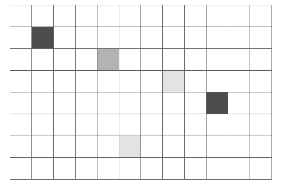
Heat “flows” between a cell and its immediate neighbors (top, bottom, left, right) at each time step. The new temperature of a grid cell is computed based on the differences between its current temperature and the temperatures of its neighbors. The update equation is as follows:

\[T_{\text{NEW}} = T_{\text{OLD}} + \sum_{\text{NEIGHBORS}} k \cdot(T_{\text{NEIGHBOR}} - T_{\text{OLD}})\]

Here, $k$ represents the rate at which heat flows through the simulation. Considering only four neighbors, the equation simplifies to:

\[T_{\text{NEW}} = T_{\text{OLD}} + k \cdot(T_{\text{TOP}} + T_{\text{BOTTOM}} + T_{\text{LEFT}} + T_{\text{RIGHT}} - 4 \cdot T_{\text{OLD}})\]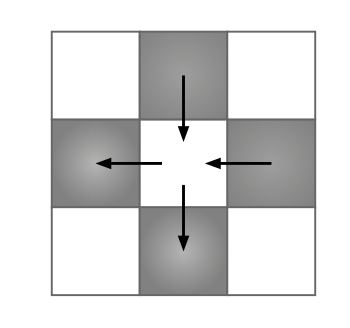

Implementing the Simulation Logic on GPU

Our heat transfer simulation involves a three-step update process, designed for efficient execution on the GPU:

1. Copy Constant Temperatures (copy_const_kernel()): Given an input temperature grid, we copy the temperatures of cells containing heaters to this grid. This step ensures that heater cells always maintain their fixed temperatures, overwriting any previously computed values in these specific locations.
2. Blend Temperatures (blend_kernel()): Using the input temperature grid, we compute the output temperatures based on the heat transfer update equation. This kernel performs the core calculation of heat distribution across the grid.
3. Buffer Swap: After computing the output temperature grid, it becomes the input for the next time step. This involves swapping the input and output buffers to prepare for the subsequent iteration.

Visualizing the Heat Transfer

To better understand the dynamic nature of the simulation, here’s a visualization of the heat transfer process:

Leveraging CUDA Texture Memory for Performance

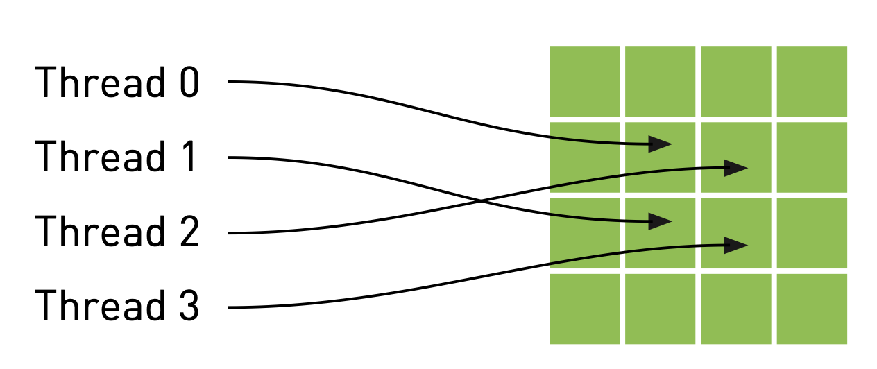
To optimize memory access patterns, especially given the spatial locality in our heat transfer calculations, we can utilize CUDA’s texture memory. Unlike general-purpose global memory (DRAM), texture memory is optimized for 2D spatial locality and features a dedicated, on-chip cache (the texture cache). This makes it particularly beneficial for applications like image processing or grid-based simulations where threads frequently access neighboring data elements. When data access patterns exhibit good spatial locality, the texture cache can significantly reduce memory latency and improve overall performance.

Threads access texture memory using specialized functions like tex1Dfetch() or tex2D(), which route memory requests through the texture unit. This unit handles the caching and addressing, allowing threads to retrieve data faster than direct global memory accesses when the access pattern aligns with texture memory’s strengths.

First, we declare our input and output buffers as texture references on the GPU side. These will be floating-point textures to accommodate our temperature data:

// these exist on the GPU side
texture<float>  texConstSrc;
texture<float>  texIn;
texture<float>  texOut;

After allocating GPU memory for our buffers, we bind these references to the memory using cudaBindTexture(). This tells the CUDA runtime to treat the specified buffer as a texture and associates it with a named texture reference:

// assume float == 4 chars in size (ie rgba)
HANDLE_ERROR( cudaMalloc( (void**)&data.dev_inSrc, imageSize ) );
HANDLE_ERROR( cudaMalloc( (void**)&data.dev_outSrc, imageSize ) );
HANDLE_ERROR( cudaMalloc( (void**)&data.dev_constSrc, imageSize ) );

HANDLE_ERROR( cudaBindTexture( NULL, texConstSrc, data.dev_constSrc, imageSize ) );
HANDLE_ERROR( cudaBindTexture( NULL, texIn, data.dev_inSrc, imageSize ) );
HANDLE_ERROR( cudaBindTexture( NULL, texOut, data.dev_outSrc, imageSize ) );

When reading from textures within a kernel, we must use special functions like tex1Dfetch() instead of direct array indexing. This routes memory requests through the texture unit. Additionally, because texture references must be declared globally, we can no longer pass input/output buffers as kernel parameters. Instead, we pass a boolean flag (dstOut) to blend_kernel() to indicate which buffer serves as input and which as output:

__global__ void blend_kernel( float *dst, bool dstOut ) {
    // map from threadIdx/BlockIdx to pixel position
    int x = threadIdx.x + blockIdx.x * blockDim.x;
    int y = threadIdx.y + blockIdx.y * blockDim.y;
    int offset = x + y * blockDim.x * gridDim.x;

    int left = offset - 1;
    int right = offset + 1;
    if (x == 0)   left++;
    if (x == DIM-1) right--; 

    int top = offset - DIM;
    int bottom = offset + DIM;
    if (y == 0)   top += DIM;
    if (y == DIM-1) bottom -= DIM;

    float   t, l, c, r, b;
    if (dstOut) {
        t = tex1Dfetch(texIn,top);
        l = tex1Dfetch(texIn,left);
        c = tex1Dfetch(texIn,offset);
        r = tex1Dfetch(texIn,right);
        b = tex1Dfetch(texIn,bottom);

    } else {
        t = tex1Dfetch(texOut,top);
        l = tex1Dfetch(texOut,left);
        c = tex1Dfetch(texOut,offset);
        r = tex1Dfetch(texOut,right);
        b = tex1Dfetch(texOut,bottom);
    }
    dst[offset] = c + SPEED * (t + b + r + l - 4 * c);
}

Similarly, copy_const_kernel() is modified to read from texConstSrc using tex1Dfetch():

__global__ void copy_const_kernel( float *iptr ) {
    // map from threadIdx/BlockIdx to pixel position
    int x = threadIdx.x + blockIdx.x * blockDim.x;
    int y = threadIdx.y + blockIdx.y * blockDim.y;
    int offset = x + y * blockIdx.x * gridDim.x;

    float c = tex1Dfetch(texConstSrc,offset);
    if (c != 0)
        iptr[offset] = c;
}

The host-side anim_gpu() routine also changes to toggle the dstOut flag instead of explicitly swapping buffers:

void anim_gpu( DataBlock *d, int ticks ) {
    HANDLE_ERROR( cudaEventRecord( d->start, 0 ) );
    dim3    blocks(DIM/16,DIM/16);
    dim3    threads(16,16);
    CPUAnimBitmap  *bitmap = d->bitmap;

    // since tex is global and bound, we have to use a flag to
    // select which is in/out per iteration
    volatile bool dstOut = true;
    for (int i=0; i<90; i++) {
        float   *in, *out;
        if (dstOut) {
            in  = d->dev_inSrc;
            out = d->dev_outSrc;
        } else {
            out = d->dev_inSrc;
            in  = d->dev_outSrc;
        }
        copy_const_kernel<<<blocks,threads>>>( in );
        blend_kernel<<<blocks,threads>>>( out, dstOut );
        dstOut = !dstOut;
    }
    float_to_color<<<blocks,threads>>>( d->output_bitmap,
                                        d->dev_inSrc );

    HANDLE_ERROR( cudaMemcpy( bitmap->get_ptr(),
                              d->output_bitmap,
                              bitmap->image_size(),
                              cudaMemcpyDeviceToHost ) );

    HANDLE_ERROR( cudaEventRecord( d->stop, 0 ) );
    HANDLE_ERROR( cudaEventSynchronize( d->stop ) );
    float   elapsedTime;
    HANDLE_ERROR( cudaEventElapsedTime( &elapsedTime,
                                        d->start, d->stop ) );
    d->totalTime += elapsedTime;
    ++d->frames;
    printf( "Average Time per frame:  %3.1f ms\n",
            d->totalTime/d->frames  );
}

Finally, remember to unbind textures during cleanup:

void anim_exit( DataBlock *d ) {
    cudaUnbindTexture( texIn );
    cudaUnbindTexture( texOut );
    cudaUnbindTexture( texConstSrc );
    HANDLE_ERROR( cudaFree( d->dev_inSrc ) );
    HANDLE_ERROR( cudaFree( d->dev_outSrc ) );
    HANDLE_ERROR( cudaFree( d->dev_constSrc ) );

    HANDLE_ERROR( cudaEventDestroy( d->start ) );
    HANDLE_ERROR( cudaEventDestroy( d->stop ) );
}

Enhancing with 2D Texture Memory

For 2D domains like our heat grid, using two-dimensional texture memory can simplify kernel code. We declare 2D textures by adding a dimensionality argument:

// these exist on the GPU side
texture<float,2>  texConstSrc;
texture<float,2>  texIn;
texture<float,2>  texOut;

The blend_kernel() and copy_const_kernel() then use tex2D() calls, directly addressing the texture with x and y coordinates, eliminating the need for linearized offsets and simplifying boundary handling (as tex2D() handles out-of-bounds access by clamping to the edge):

__global__ void blend_kernel( float *dst,
                              bool dstOut ) {
    // map from threadIdx/BlockIdx to pixel position
    int x = threadIdx.x + blockIdx.x * blockDim.x;
    int y = threadIdx.y + blockIdx.y * blockDim.y;
    int offset = x + y * blockIdx.x * gridDim.x;

    float   t, l, c, r, b;
    if (dstOut) {
        t = tex2D(texIn,x,y-1);
        l = tex2D(texIn,x-1,y);
        c = tex2D(texIn,x,y);
        r = tex2D(texIn,x+1,y);
        b = tex2D(texIn,x,y+1);
    } else {
        t = tex2D(texOut,x,y-1);
        l = tex2D(texOut,x-1,y);
        c = tex2D(texOut,x,y);
        r = tex2D(texOut,x+1,y);
        b = tex2D(texOut,x,y+1);
    }
    dst[offset] = c + SPEED * (t + b + r + l - 4 * c);
}

__global__ void copy_const_kernel( float *iptr ) {
    // map from threadIdx/BlockIdx to pixel position
    int x = threadIdx.x + blockIdx.x * blockDim.x;
    int y = threadIdx.y + blockIdx.y * blockDim.y;
    int offset = x + y * blockIdx.x * gridDim.x;

    float c = tex2D(texConstSrc,x,y);
    if (c != 0)
        iptr[offset] = c;
}

When binding 2D textures, we use cudaBindTexture2D() and must provide a cudaChannelFormatDesc:

// assume float == 4 chars in size (ie rgba)
HANDLE_ERROR( cudaMalloc( (void**)&data.dev_inSrc, imageSize ) );
HANDLE_ERROR( cudaMalloc( (void**)&data.dev_outSrc, imageSize ) );
HANDLE_ERROR( cudaMalloc( (void**)&data.dev_constSrc, imageSize ) );

cudaChannelFormatDesc desc = cudaCreateChannelDesc<float>();
HANDLE_ERROR( cudaBindTexture2D( NULL, texConstSrc, data.dev_constSrc, desc, DIM, DIM, sizeof(float) * DIM ) );

HANDLE_ERROR( cudaBindTexture2D( NULL, texIn, data.dev_inSrc, desc, DIM, DIM, sizeof(float) * DIM ) );

HANDLE_ERROR( cudaBindTexture2D( NULL, texOut, data.dev_outSrc, desc, DIM, DIM, sizeof(float) * DIM ) );

Setting Up Your Cloud Environment (GCP & X11)

To run and visualize your CUDA simulation, you’ll need a GPU-enabled virtual machine in the cloud and a way to display its graphical output locally.

1. Provision a GPU VM on Google Cloud

You can quickly spin up a VM with an NVIDIA Tesla T4 GPU and pre-installed CUDA using a gcloud command. For detailed instructions on this setup, refer to my previous post: “Launch a Google Cloud GPU VM and Run CUDA in Under 10 Minutes”. Once your VM is running, note its External IP.

2. Connect Seamlessly with VS Code Remote SSH

For a smooth development experience, connect to your VM using VS Code’s Remote - SSH extension. First, ensure SSH works from your local terminal:

gcloud compute ssh instance-20250621-104916 --zone us-central1-f

Then, configure your ~/.ssh/config for easy VS Code access:

Host cuda-lab
  HostName <EXTERNAL_IP>
  User <YOUR_GCP_USERNAME>
  IdentityFile ~/.ssh/google_compute_engine

In VS Code, install the Remote - SSH extension, open the Remote Explorer, and connect to cuda-lab. Confirm your GPU is online with nvidia-smi.

3. Compile and Run Your CUDA Program

Once connected, compile your CUDA code (e.g., heat.cu) using nvcc:

nvcc -o heat_simulation heat.cu -lGL -lGLU -lglut
./heat_simulation

4. Run CUDA GUI Apps Remotely with X11 Forwarding

To display the graphical output of your simulation on your local Mac, you’ll use X11 forwarding:

1. Install XQuartz:

   brew install --cask xquartz
   

2. Configure XQuartz: Run open -a XQuartz. Go to XQuartz Preferences -> Security -> check “Allow connections from network clients”.
3. Set DISPLAY variable locally:

   export DISPLAY=:0
   

4. SSH with X11 forwarding:

   ssh -Y username@remote_vm_ip
   

5. **Verify X11 forwarding (on remote VM):

   echo $DISPLAY
   xeyes # A simple test application
   

   Now, when you run your compiled CUDA program (./heat_simulation) on the remote VM, its graphical output should appear on your local machine.

Conclusion

Simulating physical phenomena like heat transfer on GPUs offers immense computational advantages. By combining CUDA programming with cloud computing resources like Google Cloud and remote visualization via X11 forwarding, you can establish a powerful and flexible development environment for high-performance applications. This workflow allows you to iterate quickly on complex simulations without the overhead of managing local GPU hardware, bringing your scientific and engineering ideas to life with unprecedented speed and visual clarity.

---

What are your thoughts? Feel free to discuss in the comments below or connect with me on LinkedIn.