Accuracy vs Precision in Algorithmic Trading Using Machine Learning Models
When developing machine learning (ML) models for algorithmic trading, one of the key challenges is determining the trade-off between accuracy and precision. Accuracy measures the overall correctness of predictions, while precision focuses on the relationship between true positives (money-making bets) and false positives (money-losing bets). This trade-off directly influences the expected Sharpe ratio, which is critical for assessing the risk-adjusted return of a trading strategy. By analyzing the outcomes of market bets within specific time windows, practitioners can identify target metrics to optimize both model training and validation.
Let’s delve into this concept by considering a trading strategy that produces $n$ independent and identically distributed (IID) bets per year. Each bet’s outcome $X_i$, where $i \in [1, n]$, is defined as follows:
- A profit $\pi > 0$ with probability $P[X_i = \pi] = p$
- A loss $-\pi$ with probability $P[X_i = -\pi] = 1 - p$
Here, $p$ can be thought of as the precision of a binary classifier:
- Positive outcomes indicate betting on an opportunity.
- Negative outcomes mean passing on an opportunity.
True positives are rewarded, false positives are punished, and negatives (whether true or false) have no direct impact. Importantly, this framework allows us to compute the expected moments per bet.
Expected Profit and Variance per Bet
The expected profit $E[X_i]$ from one bet is: \(E[X_i] = \pi p + (-\pi)(1 - p) = \pi (2p - 1)\)
The variance $V[X_i]$ of a single bet is derived as follows:
The second moment $E[X_i^2]$: \(E[X_i^2] = \pi^2 p + (-\pi)^2 (1 - p) = \pi^2\)
The variance: \(V[X_i] = E[X_i^2] - E[X_i]^2 = \pi^2 - \pi^2 (2p - 1)^2 = \pi^2 [1 - (2p - 1)^2] = 4\pi^2 p (1 - p)\)
Annualized Sharpe Ratio
For $n$ IID bets per year, the annualized Sharpe ratio $\theta[p, n]$ is given by: \(\theta[p, n] = \frac{n E[X_i]}{\sqrt{n V[X_i]}} = \frac{2p - 1}{2\sqrt{p(1 - p)}} \sqrt{n}\)
This equation illustrates several key insights:
- The parameter $\pi$ cancels out, highlighting that the Sharpe ratio depends only on $p$ and $n$.
- $\theta[p, n]$ can be interpreted as a re-scaled t-value, similar to statistical hypothesis testing under $H_0: p = 1/2$.
Symmetrical Payout and Its Implications
In this framework, the expected profit per bet is symmetrical, meaning the payout for winning bets is $+\pi$, while the loss for losing bets is $-\pi$. This symmetry ensures that the parameter $\pi$ cancels out when calculating key metrics like the Sharpe ratio.
For example, consider a precision of $p = 0.55$: \(\theta[p, n] = \frac{2p - 1}{2\sqrt{p(1 - p)}} \sqrt{n}\) Substituting $p = 0.55$, we get: \(\frac{2(0.55) - 1}{2\sqrt{0.55(1 - 0.55)}} \approx 0.1005\) To achieve an annualized Sharpe ratio of $\theta = 2$, the required number of bets per year is: \(n = \left(\frac{\theta \cdot 2\sqrt{p(1 - p)}}{2p - 1}\right)^2 = \left(\frac{2 \cdot 2\sqrt{0.55 \cdot 0.45}}{2(0.55) - 1}\right)^2 \approx 396\)
This shows that even modest precision levels can yield high Sharpe ratios if the betting frequency $n$ is sufficiently high.
Trade-off Between Precision and Frequency
The relationship between precision $p$, frequency $n$, and Sharpe ratio $\theta$ can be explicitly expressed as: \(-4p^2 + 4p - \frac{n}{\theta^2 + n} = 0\) Solving for $p$, we obtain: \(p = \frac{1}{2} \left(1 + \sqrt{1 - \frac{n}{\theta^2 + n}}\right)\)
This equation highlights the trade-off between $p$ and $n$ for a given Sharpe ratio $\theta$. For example, a strategy that only produces weekly bets ($n = 52$) would require a precision of: \(p = \frac{1}{2} \left(1 + \sqrt{1 - \frac{52}{2^2 + 52}}\right) \approx 0.6336\)
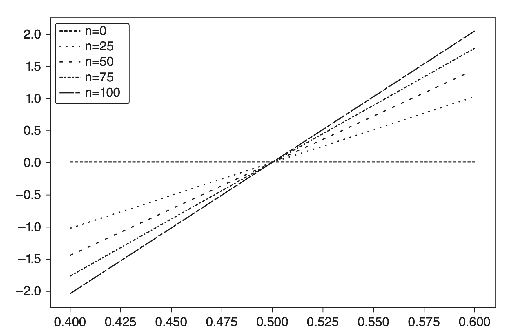
The figure below illustrates this trade-off, showing the Sharpe ratio as a function of precision for various betting frequencies. High frequencies ($n$) can compensate for lower precision, while lower frequencies demand higher precision to achieve similar Sharpe ratios.
By understanding this interplay, practitioners can align their strategy’s design with the operational constraints of their trading environment, balancing precision and frequency to optimize performance.
Implications for Algorithmic Trading
Even for small values of $p > 1/2$, the Sharpe ratio can be significantly increased by raising $n$. This underscores the economic foundation of high-frequency trading, where precision $p$ may be only slightly above 50%, but the sheer volume of bets $n$ drives profitability.
The Sharpe ratio is a function of precision rather than accuracy because passing on opportunities (negatives) does not directly affect rewards or penalties. However, too many negatives can reduce $n$, ultimately depressing the Sharpe ratio toward zero.
Conclusion
Understanding the interplay between accuracy and precision is crucial for developing effective ML models in algorithmic trading. While accuracy measures overall correctness, precision focuses on the quality of positive predictions—a critical factor for boosting the Sharpe ratio. By aligning model training and validation with these metrics, practitioners can design strategies that maximize profitability and robustness in trading environments.
