Visual Intuition Behind Jensen Inquality

Jensen’s inequality forms a cornerstone of probability theory and convex analysis, establishing a relationship between the expected value of a function and the function of an expected value. The mathematical formulation states that for a convex function $\varphi$ and a random variable $X$:

\[\varphi(\mathbb{E}[X]) \leq \mathbb{E}[\varphi(X)]\]

This inequality has profound implications in statistics, inftyormation theory, and financial mathematics. Understanding its geometric interpretation provides deeper insights into why this relationship holds true and its practical applications.

Geometric Interpretation

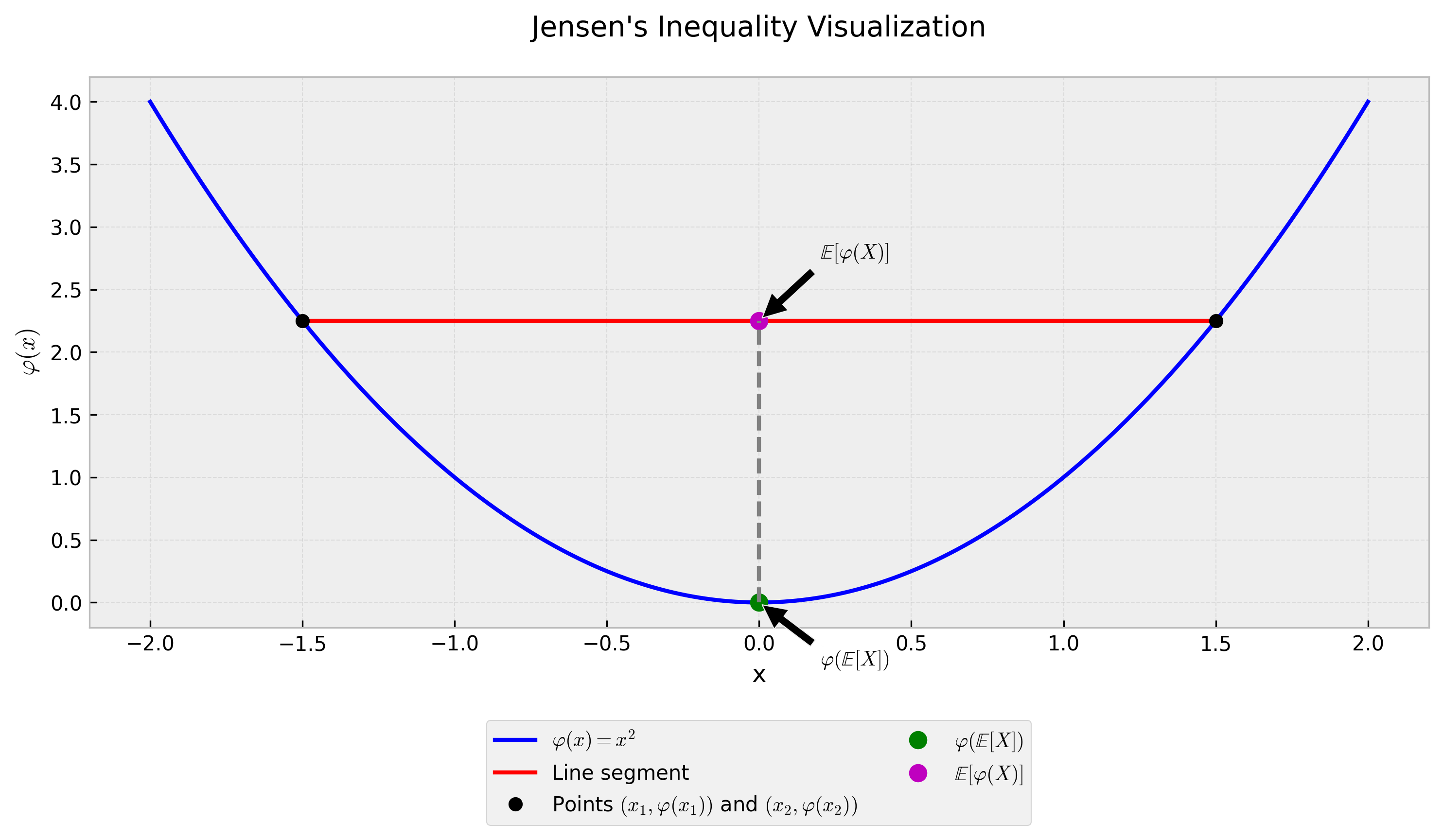
The geometric interpretation of Jensen’s inequality emerges from the definition of convex functions. A function is convex when a line segment between any two points on its graph lies above or on the graph. For a convex function $\varphi(x)$, consider two points $x_1$ and $x_2$. The weighted average of their function values will always be greater than or equal to the function value of their weighted average.

In the visualization above, the blue curve represents a convex function $\varphi(x)$. The red line segment connects two points $(x_1, \varphi(x_1))$ and $(x_2, \varphi(x_2))$. Any point on this line segment represents a weighted average of the function values, while the corresponding point on the curve represents the function value of the weighted average of $x_1$ and $x_2$.

Mathematical Foundation

The inequality’s power extends beyond simple weighted averages to expectations of random variables. For a continuous random variable X with probability density function f(x), Jensen’s inequality states:

\[\varphi \left(\int_{-\infty}^{\infty} x f(x) dx \right) \leq \int_{-\infty}^{\infty} \varphi(x) f(x) dx\]

This formulation demonstrates that the expected value of a convex function applied to a random variable is greater than or equal to the function applied to the expected value of the random variable.

Applications in Finance and Statistics

Jensen’s inequality explains numerous phenomena in quantitative finance and statistics:

The inequality explains why the geometric mean of returns is always less than or equal to the arithmetic mean. For a log-normal distribution of asset returns, this relationship becomes:

\[\mathbb{E}[\ln(1 + R)] \leq \ln(1 + \mathbb{E}[R])\]

This inequality impacts portfolio management, particularly in understanding the difference between arithmetic and geometric returns. Long-term investors must account for this effect when projecting future portfolio values.

In risk management, Jensen’s inequality explains why variance and other higher moments of return distributions affect long-term compound returns. The convexity of the exponential function leads to:

\[\mathbb{E}[e^X] \geq e^{\mathbb{E}[X]}\]

This relationship becomes crucial when dealing with options pricing and risk-neutral valuation, where the convexity of payoff functions plays a central role.

Practical Implications

Understanding Jensen’s inequality helps practitioners in several ways:

The inequality explains why diversification reduces portfolio risk. The convexity of variance means that the variance of a portfolio is less than or equal to the weighted average of individual asset variances.

In machine learning, the inequality underlies the effectiveness of ensemble methods. The convexity of error functions means that averaging predictions often produces better results than individual models.

For time series analysis, the inequality helps understand why geometric averaging provides a more accurate measure of long-term growth rates compared to arithmetic averaging.

Computational Verification

We can verify Jensen’s inequality computationally using Python:

import numpy as np
import matplotlib.pyplot as plt

# Define a convex function (e.g., x^2)
def convex_function(x):
    return x**2

# Generate random points
x = np.linspace(-2, 2, 1000)
y = convex_function(x)

# Calculate expected value and function value
points = np.array([-1, 1])  # Two points for demonstration
expected_value = np.mean(points)
expected_function = convex_function(expected_value)
function_expected = np.mean([convex_function(p) for p in points])

print(f"\\varphi(\\mathbb[X]) = {expected_function:.4f}")
print(f"\\mathbb[\\varphi(X)] = {function_expected:.4f}")

The computational example demonstrates that $\mathbb{E}[\varphi(X)]$ consistently exceeds or equals $\varphi(\mathbb{E}[X])$ for our convex function, confirming the theoretical inequality.

Jensen’s inequality provides a fundamental tool for understanding relationships between expectations and nonlinear transformations. Its visual interpretation offers intuitive insights into why these relationships hold true across various domains in quantitative analysis.

---